OCR tables and parse the output
In this tutorial, we will illustrate how easily the layoutparser
APIs can be used for
Recognizing texts in images and store the results with the specified OCR engine
Postprocessing of the textual results to create structured data
import layoutparser as lp

import matplotlib.pyplot as plt
%matplotlib inline

import pandas as pd
import numpy as np
import cv2
Initiate GCV OCR engine and check the image
Currently, layoutparser supports two types of OCR engines: Google
Cloud Vision and Tesseract OCR engine. And we are going to provide more
support in the future. In this toturial, we will use the Google Cloud
Vision engine as an example.
ocr_agent = lp.GCVAgent.with_credential("<path/to/your/credential>",
                                       languages = ['en'])
The language_hints tells the GCV which langeuage shall be used for
OCRing. For a detailed explanation, please check
here.
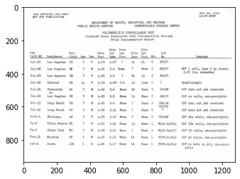
The example-table is a scan with complicated table structures from
https://stacks.cdc.gov/view/cdc/42482/.
image = cv2.imread('data/example-table.jpeg')
plt.imshow(image);
Load images and send for OCR
The ocr_agent.detect method can take the image array, or simply the
path of the image, for OCR. By default it will return the text in the
image, i.e., text = ocr_agent.detect(image).
However, as the layout is complex, the text information is not enough:
we would like to directly analyze the response from GCV Engine. We can
set the return_response to True. This feature is also supported
for other OCR Engines like TesseractOCRAgent.
res = ocr_agent.detect(image, return_response=True)

# Alternative
# res = ocr_agent.detect('data/example-table.jpeg', return_response=True)
Parse the OCR output and visualize the layout
As defined by GCV, there are two different types of output in the response:
text_annotations:
In this format, GCV automatically find the best aggregation level for the text, and return the results in a list. We canuse theocr_agent.gather_text_annotationsto reterive this type of information.full_text_annotations
To support better user control, GCV also provides the
full_text_annotationoutput, where it returns the hierarchical structure of the output text. To process this output, we provide theocr_agent.gather_full_text_annotationfunction to aggregate the texts of the given aggregation level.There are 5 levels specified in
GCVFeatureType, namely:PAGE,BLOCK,PARA,WORD,SYMBOL.
texts  = ocr_agent.gather_text_annotations(res)
    # collect all the texts without coordinates
layout = ocr_agent.gather_full_text_annotation(res, agg_level=lp.GCVFeatureType.WORD)
    # collect all the layout elements of the `WORD` level
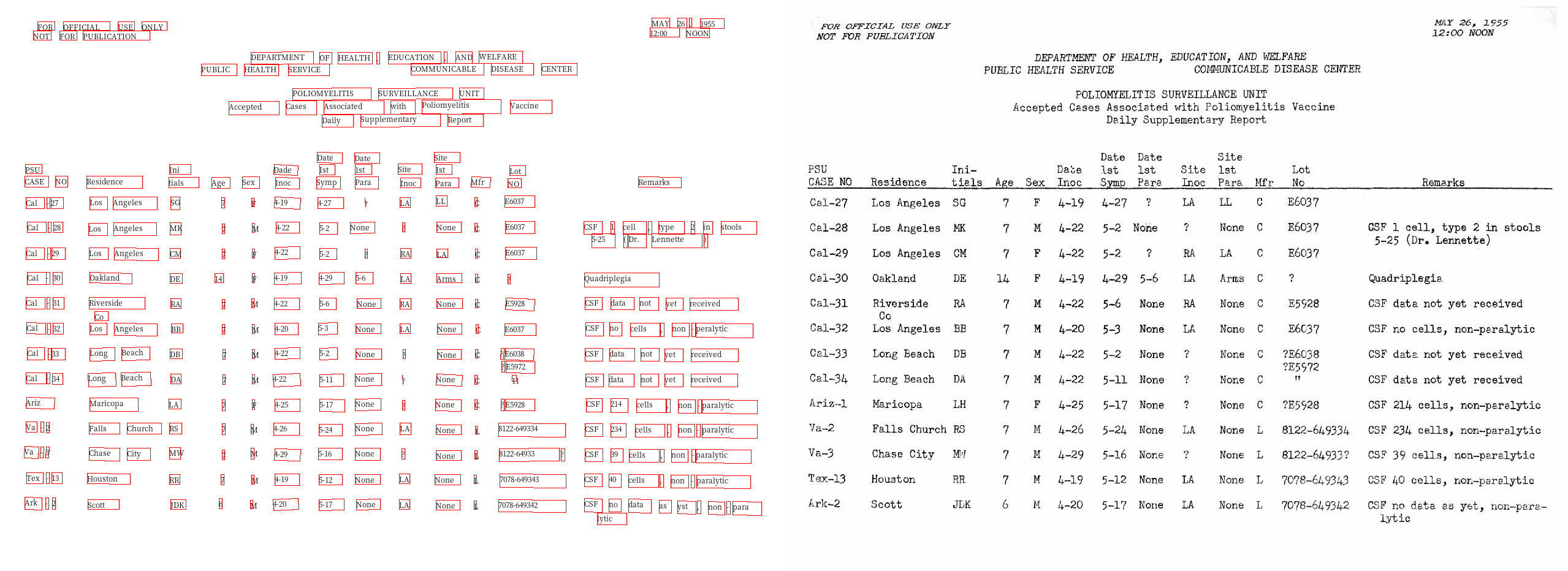
And we can use the draw_box or draw_text functions to quickly
visualize the detected layout and text information.
These functions are highly customizable. You can change styles of the drawn boxes and texts easily. Please check the documentation for the detailed explanation of the configurable parameters.
As shown below, the draw_text function generates a visualization
that:
it draws the detected layout with text on the left side and shows the original image on the right canvas for comparison.
on the text canvas (left), it also draws a red bounding box for each text region.
lp.draw_text(image, layout, font_size=12, with_box_on_text=True,
             text_box_width=1)
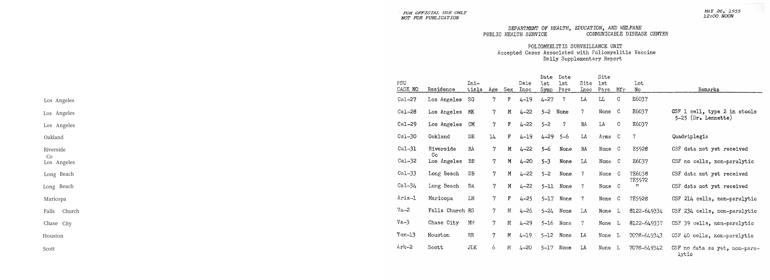
Filter the returned text blocks
We find the coordinates of residence column are in the range of
\(y\in(300,833)\) and \(x\in(132, 264)\). The
layout.filter_by function can be used to fetch the texts in the
region.
Note: As the OCR engine usually does not provide advanced functions like table detection, the coordinates are found manually by using some image inspecting tools like GIMP.
filtered_residence = layout.filter_by(
    lp.Rectangle(x_1=132, y_1=300, x_2=264, y_2=840)
)
lp.draw_text(image, filtered_residence, font_size=16)
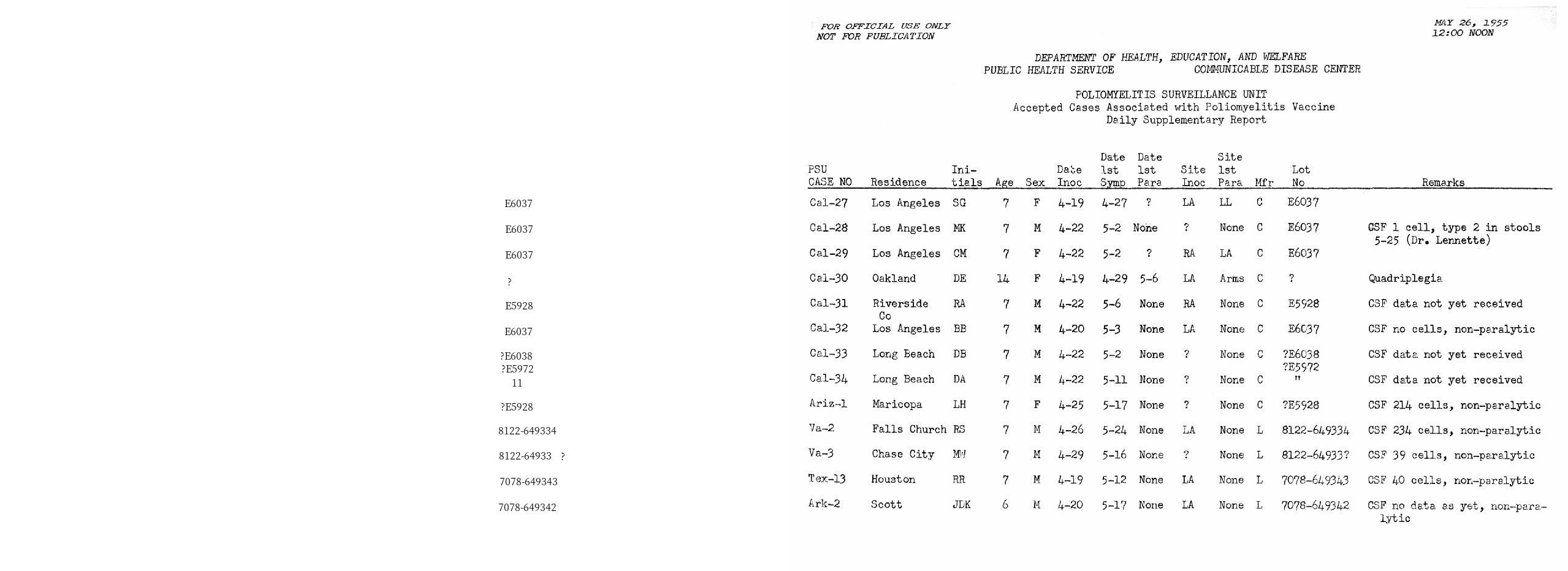
And similarily, we can do that for the lot_number column. As
sometimes there could be irregularities in the layout as well as the OCR
outputs, the layout.filter_by function also supports a
soft_margin argument to handle this issue and generate more robust
outputs.
filter_lotno = layout.filter_by(
    lp.Rectangle(x_1=810, y_1=300, x_2=910, y_2=840),
    soft_margin = {"left":10, "right":20} # Without it, the last 4 rows could not be included
)
lp.draw_text(image, filter_lotno, font_size=16)
Group Rows based on hard-coded parameteres
As there are 13 rows, we can iterate the rows and fetch the row-based information:
y_0 = 307
n_rows = 13
height = 41
y_1 = y_0+n_rows*height

row = []
for y in range(y_0, y_1, height):

    interval = lp.Interval(y,y+height, axis='y')
    residence_row = filtered_residence.\
        filter_by(interval).\
        get_texts()

    lotno_row = filter_lotno.\
        filter_by(interval).\
        get_texts()

    row.append([''.join(residence_row), ''.join(lotno_row)])
row
[['LosAngeles', 'E6037'],
 ['LosAngeles', 'E6037'],
 ['LosAngeles', 'E6037'],
 ['Oakland', '?'],
 ['Riverside', 'E5928'],
 ['LosAngeles', 'E6037'],
 ['LongBeach', '?E6038'],
 ['LongBeach', '11'],
 ['Maricopa', '?E5928'],
 ['FallsChurch', '8122-649334'],
 ['ChaseCity', '8122-64933?'],
 ['Houston', '7078-649343'],
 ['Scott', '7078-649342']]
An Alternative Method - Adaptive Grouping lines based on distances
blocks = filter_lotno

blocks = sorted(blocks, key = lambda x: x.coordinates[1])
    # Sort the blocks vertically from top to bottom
distances = np.array([b2.coordinates[1] - b1.coordinates[3] for (b1, b2) in zip(blocks, blocks[1:])])
    # Calculate the distances:
    # y coord for the upper edge of the bottom block -
    #   y coord for the bottom edge of the upper block
    # And convert to np array for easier post processing
plt.hist(distances, bins=50);
plt.axvline(x=3, color='r');
    # Let's have some visualization
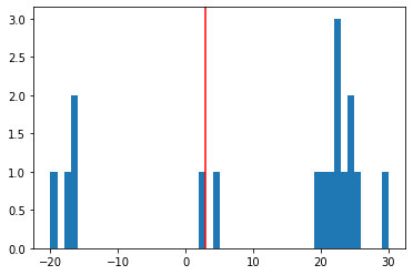
According to the distance distribution plot, as well as the OCR results visualization, we can conclude:
For the negative distances, it’s because there are texts in the same line, e.g., “Los Angeles”
For the small distances (indicated by the red line in the figure), they are texts in the same table row as the previous one
For larger distances, they are generated from texts pairs of different rows
distance_th = 0

distances = np.append([0], distances) # Append a placeholder for the first word
block_group = (distances>distance_th).cumsum() # Create a block_group based on the distance threshold

block_group
array([ 0,  1,  2,  3,  4,  5,  6,  6,  7,  7,  8,  9,  9, 10, 11, 11, 12,
       13])
# Group the blocks by the block_group mask
grouped_blocks = [[] for i in range(max(block_group)+1)]
for i, block in zip(block_group, blocks):
    grouped_blocks[i].append(block)
Finally let’s create a function for them
def group_blocks_by_distance(blocks, distance_th):

    blocks = sorted(blocks, key = lambda x: x.coordinates[1])
    distances = np.array([b2.coordinates[1] - b1.coordinates[3] for (b1, b2) in zip(blocks, blocks[1:])])

    distances = np.append([0], distances)
    block_group = (distances>distance_th).cumsum()

    grouped_blocks = [lp.Layout([]) for i in range(max(block_group)+1)]
    for i, block in zip(block_group, blocks):
        grouped_blocks[i].append(block)

    return grouped_blocks
A = group_blocks_by_distance(filtered_residence, 5)
B = group_blocks_by_distance(filter_lotno, 10)

# And finally we combine the outputs
height_th = 30
idxA, idxB = 0, 0

result = []
while idxA < len(A) and idxB < len(B):
    ay = A[idxA][0].coordinates[1]
    by = B[idxB][0].coordinates[1]
    ares, bres = ''.join(A[idxA].get_texts()), ''.join(B[idxB].get_texts())
    if abs(ay - by) < height_th:
        idxA += 1; idxB += 1
    elif ay < by:
        idxA += 1; bres = ''
    else:
        idxB += 1; ares = ''
    result.append([ares, bres])

result
[['LosAngeles', 'E6037'],
 ['AngelesLos', 'E6037'],
 ['LosAngeles', 'E6037'],
 ['Oakland', '?'],
 ['RiversideCoLosAngeles', 'E5928'],
 ['', 'E6037'],
 ['BeachLong', '?E6038?E597211'],
 ['BeachLong', ''],
 ['Maricopa', '?E5928'],
 ['FallsChurch', '8122-649334'],
 ['ChaseCity', '8122-64933?'],
 ['Houston', '7078-649343'],
 ['Scott', '7078-649342']]
As we can find, there are mistakes in the 5th and 6h row -
Riverside Co and LosAngeles are wrongly combined. This is
because the extra row co disrupted the row segmentation algorithm.
Save the results as a table
df = pd.DataFrame(row, columns=['residence', 'lot no'])
df
| residence | lot no | |
|---|---|---|
| 0 | LosAngeles | E6037 |
| 1 | LosAngeles | E6037 |
| 2 | LosAngeles | E6037 |
| 3 | Oakland | ? |
| 4 | Riverside | E5928 |
| 5 | LosAngeles | E6037 |
| 6 | LongBeach | ?E6038 |
| 7 | LongBeach | 11 |
| 8 | Maricopa | ?E5928 |
| 9 | FallsChurch | 8122-649334 |
| 10 | ChaseCity | 8122-64933? |
| 11 | Houston | 7078-649343 |
| 12 | Scott | 7078-649342 |
df.to_csv('./data/ocred-example-table.csv', index=None)